Introduction
Dividend discount models (DDM) provide a basic mechanism to value companies by discounting expected dividend cash flows back to the current period. Practitioners typically assume a series of dividend growth rates over a short horizon along with a constant terminal growth rate. These assumptions imply a multi-stage model with growth rates \(g_1,\ldots,g_A\) for the first \(A\) periods, and a terminal growth rate \(g_\infty\). Given an initial dividend amount, \(D_0\), and a discount rate, \(r\), the present value today, \(P_0\), is
\[\begin{equation} P_0 = D_0 \sum_{t=1}^A \left(\dfrac{1 + g_t}{1 + r} \right)^t + D_A\dfrac{ \frac{1+g_{\infty}}{r-g_{\infty}} }{ (1 + r)^A } \tag{1} \end{equation}\]
Determining the growth rates is a tricky task. The terminal rate in particular cannot be too high, or else the second term—often called the terminal value—will be unreasonably large. Therefore, the earlier rates, \(g_1,\ldots,g_A\), are often chosen to decrease towards a lower terminal rate. In some cases, this strategy results in a cliff, where the drop from \(g_A\) to \(g_\infty\) is significant. The drop is hard to justify qualitatively, although typically accepted to arrive at a reasonable valuation.
The H-model
The H-model proposed by Fuller and Hsia (1984) seeks to alleviate these issues by assuming a linear decline in the growth rate during the first \(A\) periods, so the modeler only need choose \(g_1\) and \(g_\infty\). The model uses the following formula to determine the present value, \[\begin{equation} P_0 = \dfrac{D_0}{r - g_\infty} [(1 + g_\infty) + H(g_1 - g_\infty)] \tag{2} \end{equation}\] where \(H\) is half of the transition period—i.e., \(H=A/2\).
Equation (2) appears quite nice, almost too nice. Indeed, the H-model is only an approximation of the present value of the assumed cash flows.1 The assumption of linearly declining growth rate does not admit much simplification of Equation (1).
However, one of the goals of Fuller and Hsia (1984) is to provide a simple analytic formula for the discount rate, given a present value. That is, \[\begin{equation} r = \dfrac{D_0}{P_0}[(1 + g_\infty) + H(g_1 - g_\infty)] + g_\infty \tag{3} \end{equation}\] Although an analytic formula is not necessary with modern computing power, most financial analysts in 1984 would have found solving Equation (1) rather time-consuming. Therefore, approximation error may have been a reasonable trade-off.
Derivation
Unfortunately, Fuller and Hsia (1984) do not provide a formal derivation of the H-model in the paper. A footnote contains the dreaded words, “available from the authors.”2 However, with a bit a guess work, it’s not too difficult to figure out how they likely arrived at Equation (2).
Two-step approximation
The authors begin with a two-step model with two growth rates. Dividends grow at the initial rate (\(g_a\)) for \(A\) periods then at the terminal rate (\(g_\infty\)) for all future periods. In the two-step model, the present value is given by equation 5 in the paper, \[\begin{equation} P_0 = D_0 \sum_{t=1}^A \left(\dfrac{1+g_a}{1+r} \right)^t + D_A \sum_{t=A+1}^\infty \left(\dfrac{(1+g_\infty)^{t-A}}{(1+r)^t} \right) \tag{4} \end{equation}\] By applying the formula for a growing annuity to the first term and the formula for a growing perpetuity to the second term, the present value can be written as \[\begin{equation} P_0 = D_0 \dfrac{1+g_a}{r-g_a}\left(1 - \left(\dfrac{1+g_a}{1+r} \right)^A \right) + D_0 \left(\dfrac{1+g_a}{1+r} \right)^A \dfrac{1+g_\infty}{r-g_\infty} \tag{5} \end{equation}\] With some algebra, Equation (5) can be rearranged as \[\begin{equation} P_0 = D_0 \dfrac{1+g_a}{r-g_a}\left(1 - \left(\dfrac{1+g_a}{1+r} \right)^{A-1} \left(\dfrac{g_a-g_\infty}{r-g_\infty} \right) \right) \tag{6} \end{equation}\] which is equation 6 in the paper.
The authors claim that (6) can be approximated by \[\begin{equation} P_0 \approx \dfrac{D_0}{r-g_\infty}\left(1 + g_\infty + A(g_a - g_\infty)\right) \tag{7} \end{equation}\]
The authors do not provide any hints for the approximation, and manipulating Equation (6) is quite messy. Instead, consider how extreme values of \(g_a\) affect the “exact” present value in Equation (4). If \(g_a=g_\infty\), then the whole cash flow series is a perpetuity with constant growth, so \(P_0=\frac{D_0(1+g_\infty)}{r-g_\infty}\). If \(g_a=r\), then both terms can be considerably simplified so \(P_0=D_0A +\frac{D_0(1+g_\infty)}{r-g_\infty}\).
Now, consider linearly interpolating between these two points for (\(g_a,P_0\)): from \(\left(g_\infty,\frac{D_0(1+g_\infty)}{r-g_\infty}\right)\) to \(\left(r,D_0A+\frac{D_0(1+g_\infty)}{r-g_\infty}\right)\). The formula for a line connecting two points, \((x, f(x))\) and \((x_1, f(x_1))\), is \[\begin{equation} f(x)-f(x_1)=m(x-x_1) \end{equation}\] where \(m\) is the slope between the two points. The slope between our two points for the present value is \(\frac{D_0A}{r-g_\infty}\), so we can write the formula as \[\begin{equation} f(x) - \frac{D_0(1+g_\infty)}{r-g_\infty} = \frac{D_0A}{r-g_\infty}(x-g_\infty) \end{equation}\] \[\begin{equation} f(x) = \frac{D_0}{r-g_\infty}(1+g_\infty+A(x-g_\infty)) \end{equation}\] So, for a particular value of \(g_a\), we have the approximation \[\begin{equation} P_0 \approx f(g_a) = \frac{D_0}{r-g_\infty}(1+g_\infty+A(g_a-g_\infty)) \end{equation}\]
The authors also write the approximation as the sum of two terms, \[\begin{equation} P_0 \approx \frac{D_0}{r-g_\infty}(1+g_\infty)+ \frac{D_0}{r-g_\infty}A(g_a-g_\infty) \end{equation}\] and add the interpretation that the first term is the underlying perpetuity, while the second term is the “excess” dividend growth during the period from 0 to \(A\) which itself grows at \(g_\infty\) starting from period \(A+1\). The approximation ignores the discounting of the excess perpetuity back to time 0.
The H-model formula
From this interpretation, one may consider a linearly declining growth rate over the \(A\) period, instead of a constant \(g_a\). In that case, the “excess growth” would be halved, to \(\frac{A}{2}(g_a - g_\infty)\) (again, ignore compounding). Finally, with \(H=A/2\), we have the H-model formula, Equation (2).
Three-step approximation
The authors do not jump directly from the two-step approximation to the H-model formula in the paper. Instead, they consider a three-step model, with growth rates of \(g_a\) for \(A\) periods, then \(g_b\) for \(B-A\) periods, then \(g_\infty\) for all future periods. In this model, they claim the present value can be approximated by \[\begin{equation} P_0 \approx \frac{D_0}{r-g_\infty}(1+g_\infty+A(g_a-g_\infty)+(B-A)(g_b-g_\infty)) \end{equation}\] again without explanation.3 Unfortunately, I was not able to find a clean mathematical way to arrive at this approximation. Of course if \(g_a=g_b=r\) or \(g_a=g_b=g_\infty\), then the approximate formula matches the exact formula. However, three points are required to form the plane representing the approximation. I suspect the authors continue the geometric interpretation above that \(A(g_a-g_\infty)\) is the excess growth in the first intermediate period, so \((B-A)(g_b-g_\infty)\) is the excess growth in the second intermediate period.
Given the three-step approximation, the authors assume \(g_b = \frac{g_a+g_n}{2}\), so the approximation reduces to \[\begin{equation} P_0 \approx \frac{D_0}{r-g_\infty}\left(1+g_\infty+\frac{A+B}{2}(g_a-g_\infty)\right) \end{equation}\] Now the authors write \(H=\frac{A+B}{2}\) to arrive at what they call the H-model. The three-step approximation does not improve the accuracy of the H-model, although it shows another way to think about the underlying assumptions as being about the growth rate rather than the length of time over which the growth rate is declining.
Approximation error
Let us now examine the accuracy of the approximations, including the H-model itself as compared to the “exact” model with linearly declining growth rate over \(2H\) periods.
Two-step
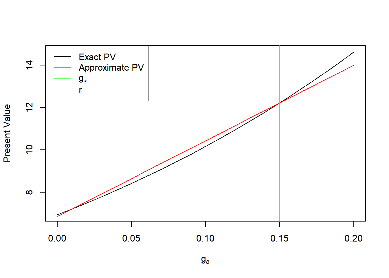
The following plot shows the present value as a function of \(g_a\) with representative values of the remaining parameters: \(D_0=1,A=5,g_\infty=0.01,r=0.15\). The lines intersect at the points used to create the approximation—that is, where \(g_a=g_\infty\) and \(g_a=r\). Interestingly, for reasonable parameter values (\(g_\infty<g_a<r\)), the approximation always overstates the present value.
Three-step
The three-step model is a bit harder to visualize, but the figure below shows the approximate present value plane represented by changing the growth rates of the first two periods, \(g_a\) and \(g_b\). The other surface is the “exact” three-step present value. The parameters were chosen to emphasize the curvature of the intersection of the surfaces: \(A=8,B=10,g_\infty=0.03,r=0.15\). Again, for typical parameters (\(g_\infty < g_a, g_b < r\)), the approximation overstates the present value.
H-model versus “exact” linear decline in growth rate
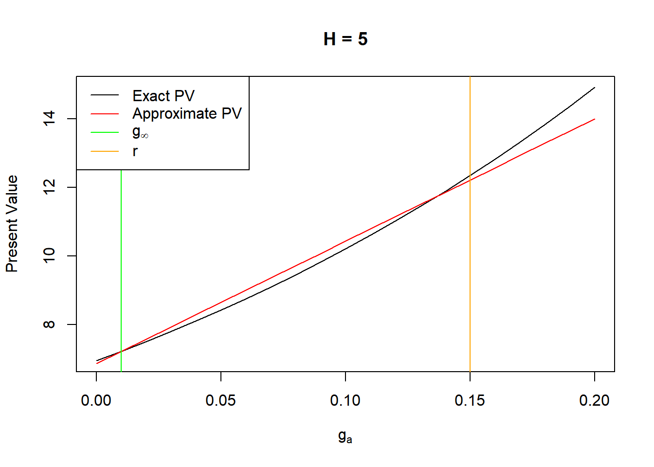
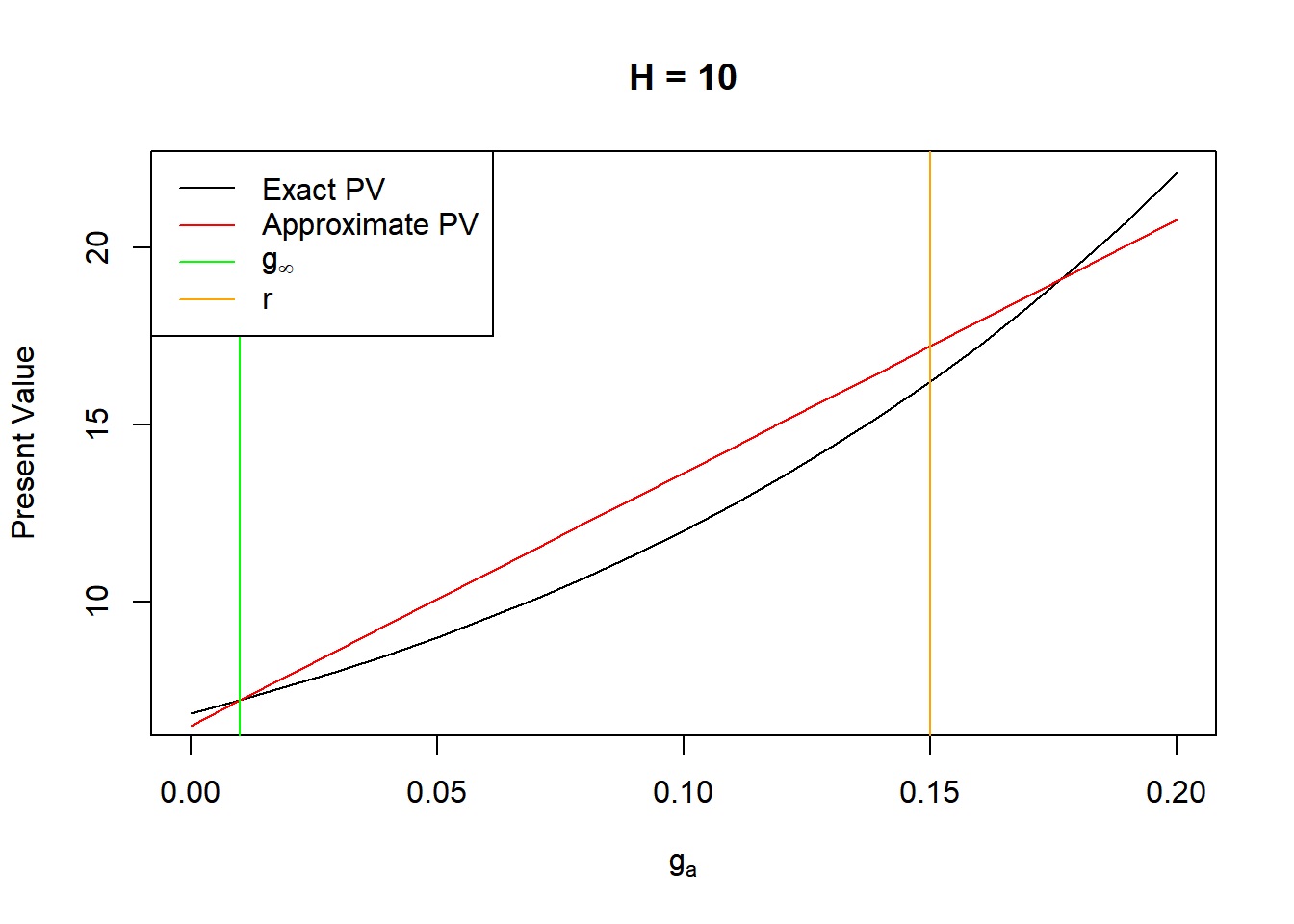
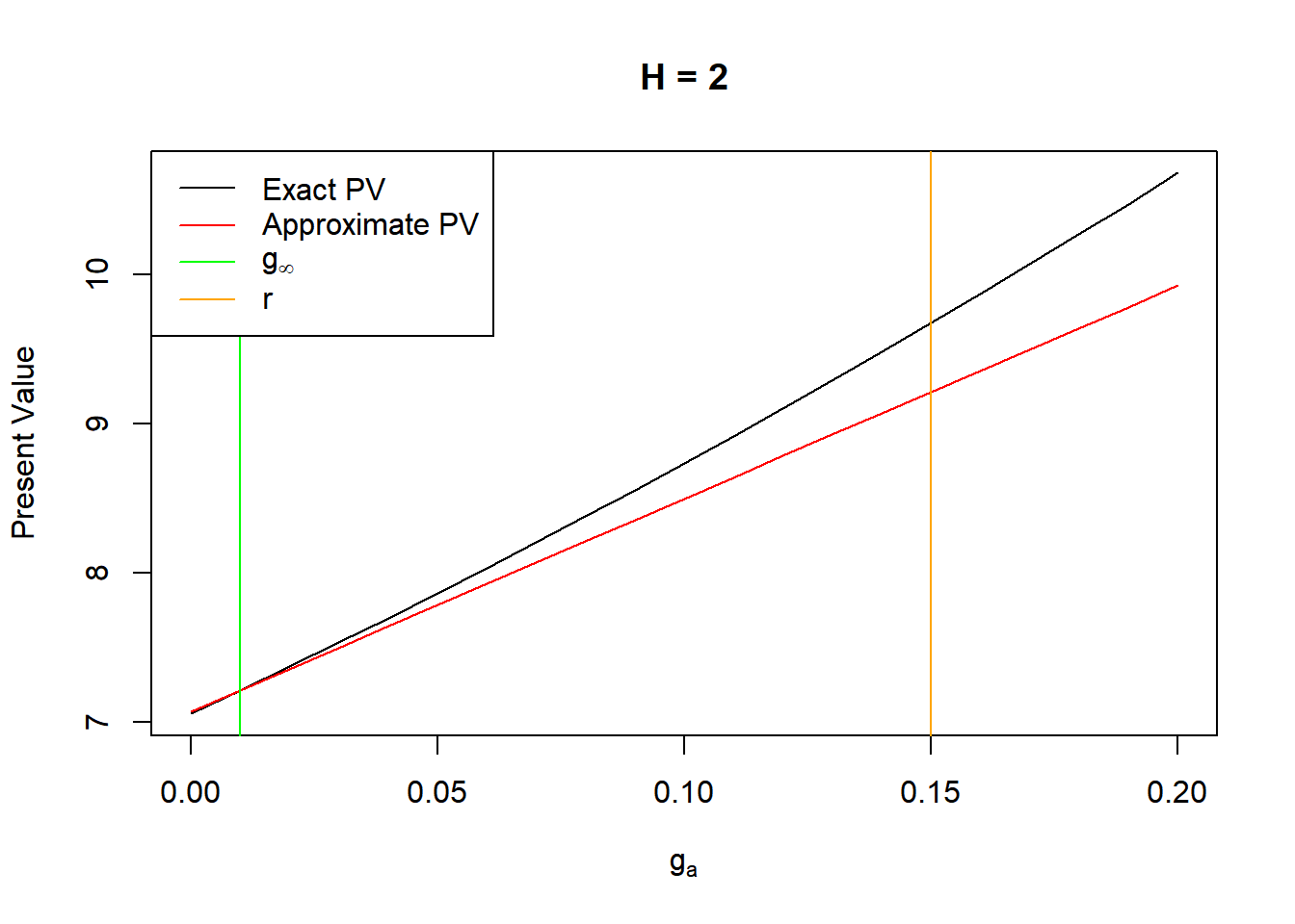
Lastly, let us compare the H-model itself to the intended underlying assumption of linearly declining growth rate over \(2H\) periods. Similar to the two-step model, the approximation is exact when \(g_a=g_\infty\), but the upper intersection point now depends on \(H\). Larger values of \(H\) tend to result in overstating the present value, while lower values the opposite.
Why did I write this post?
That’s a great question. I came across the H-model in my normal course of work. It seemed like an elegant simplification of a more general model (linearly declining growth), so I tried to work out the derivation. After unsuccessful attempts, I decided to dig up the original paper. Finding out it was only an approximation was quite annoying, doubly so when I saw the authors didn’t bother to include explanation—let alone derivation—of the approximate form.
I guess I felt committed at this point, so I spent some time trying to deduce the path from the “exact” formula to the approximate one. The two-step model eventually worked out nicely, but the three-step (or n-step) approximation appears to be heuristic.
References
Fuller, Russell J. and Chi-Cheng Hsia (1984): “A Simplified Common Stock Valuation Model,” Financial Analysts Journal, Sep.–Oct., 1984, Vol. 40, No. 5, pp. 49–56. https://www.jstor.org/stable/4478774
Many online resources explaining the H-model omit this important detail. The subjective choices of the growth and discount rates dwarf the materiality of approximation error, but it’s nonetheless important for practitioners to understand how the model works.↩︎
If you are unfamiliar with academic writing, this means it’s not available. If it were available, it would be in the paper.↩︎
In a footnote, they claim a general approximation for \(N\) intermediate growth periods of the form \(\frac{D_0}{r-g_\infty}(1+g_\infty+X_1(g_1-g_\infty)+X_2(g_2-g_\infty)+\ldots. +X_N(g_N-g_\infty))\), where \(X_i\) is the length of each period.↩︎